Analysis Tools¶

Plotting Features¶

Todo

More info coming soon.

Atomic and Molecular Lines¶

Search atomic and molecular lines from the following databases:

NIST (download1): atomic lines

HITEMP (download2, paper2): molecular lines H2O, CO2, CO, NO, and OH

APOGEE (download3, paper3): atomic and molecular lines

Functions¶

Search what line libraries are available, and what lists of elements/molecules are stored in each:

 >> import apogee_tools as ap

 >> ap.listLibraries()
    ['APOGEE_MOLEC', 'SOUTO', 'APOGEE_ATOMS', 'HITEMP', 'NIST']

 >> ap.listSpecies('APOGEE_ATOMS')
    ['CC', 'CN', 'CO', 'HH', 'OH', 'SIH']

 >> ap.listSpecies('SOUTO'))
    ['Al I', 'Ca I', 'Cr I', 'Fe I', 'FeH', 'K I', 'Mg I', 'Mn I',
'Na I', 'OH', 'Si I', 'Ti I', 'TiO', 'V I'], dtype='<U4')

 >> ap.listSpecies('APOGEE_ATOMS')
    ['AL I', 'AL II', 'AR I', 'AR II', 'AR III', 'AU I', 'B I', 'B II',
    'C I', 'C II', 'C III', 'CA I', 'CA II', 'CA III', 'CE III',
    'CL I', 'CL II', 'CL III', 'CO I', 'CO II', 'CR I', 'CR II',
    'CR III', 'CS I', 'CU I', 'CU II', 'F I', 'F II', 'F III', 'FE I',
    'FE II', 'FE III', 'GE I', 'HE I', 'K I', 'K III', 'LI I', 'MG I',
    'MG II', 'MN I', 'MN II', 'MN III', 'N I', 'N II', 'N III', 'NA I',
    'NE I', 'NE II', 'NI I', 'NI II', 'NI III', 'O I', 'O II', 'O III',
    'P I', 'P II', 'P III', 'RB I', 'S I', 'S II', 'SC I', 'SC II',
    'SC III', 'SI I', 'SI II', 'SI III', 'SR II', 'TI I', 'TI II',
    'TI III', 'V I', 'V II', 'V III', 'Y I', 'Y II', 'ZN III']

 >> ap.listSpecies('HITEMP')
    ['CO', 'CO2', 'H2O', 'NO', 'OH']

Search a wavelegth region for certain species of atoms/molecules (returns a dictionary):

>> lines = ap.searchLines(species=['OH', 'Fe I'], range=[15200,15210], \
           libraries=['NIST', 'APOGEE_ATOMS', 'APOGEE_MOLEC', 'HITEMP'])

   {'Fe I': array([15201.822, 15202.952,     0.   , 15207.106, 15208.251]),
    'OH': array([15200.214     , 15200.332     , 15201.556     , 15201.774     ,
037     , 15202.215     , 15202.296     , 15202.366     ,
93      , 15203.768     , 15203.908     , 15203.98      ,
371     , 15204.548     , 15205.168     , 15206.303     ,
019     , 15207.416     , 15207.546     , 15207.659     ,
254     , 15208.613     , 15209.474     , 15200.68827257,
3097307 , 15202.31102492, 15202.53883371, 15204.0112159 ,
21089622, 15204.31956908, 15205.52045337, 15205.71449241,
01852145, 15206.27113677, 15206.33572209, 15206.51148174,
09644387, 15207.93042108, 15208.05808934, 15208.06268267,
125648  , 15208.34296383, 15208.8060811 ])}

Example¶

How to identify lines in an APOGEE spectrum:

Read in a the spectrum of a source, and interpolate the spectrum using a spline function to determine where the max/min points are:

>> spec = ap.Apogee(id='2M19213157+4317347', type='aspcap')
>> spec = ap.rvShiftSpec(spec, rv=-80)
>> spec.name = '2M19213157+4317347'

>> interp, local_min, local_max = ap.splineInterpolate(spec)
>> min_lines = {'min':np.array(local_min)}

Create a list of species that you want to search for.

For example to search for Fe I, Ca I, Mg I and K I:

>> fe = ['Fe I', 'FE I']
>> mg = ['Mg I', 'MG I']
>> ca = ['Ca I', 'CA I']
>> k  = ['K I', 'K I']

>> species = fe + mg + ca + k

or to search for all of the species in all of the libraries:

>> species = sum([ap.listSpecies(lib) for lib in ap.listLibraries()], [])

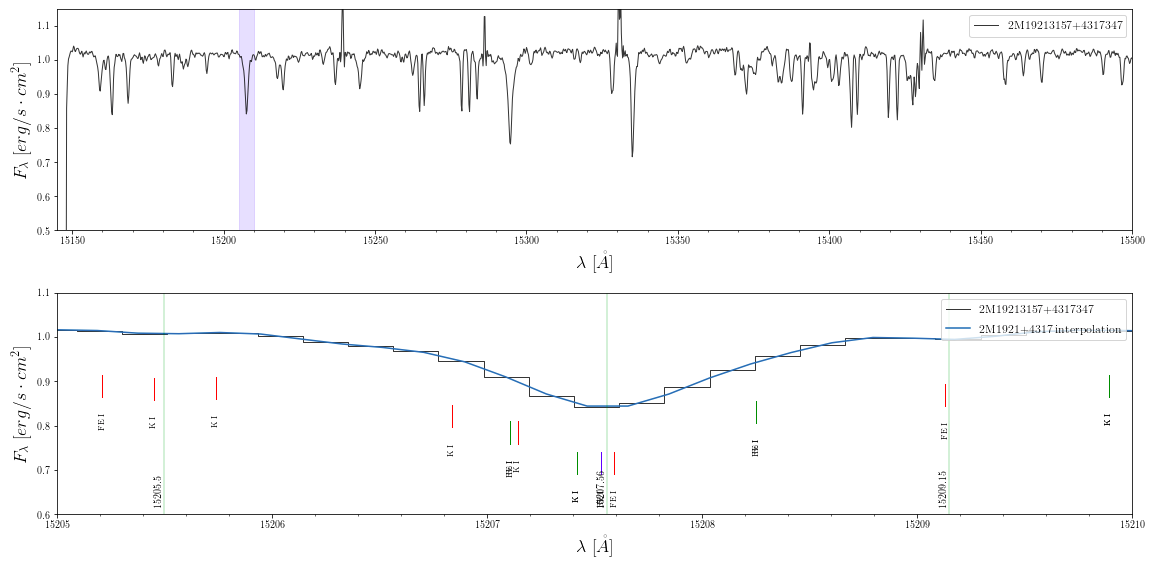
Now choose the line lists you want to search and plot the spectrum. Pick a wavelength region with a feature to zoom onto. Here the green lines mark the minimum points from the interpolated spectrum. For example searching for species Fe I, Ca I, Mg I and K I returns:

>> broad = [15145,15500]
>> zoom  = [15205,15210]

>> lines1 = ap.searchLines(species=species, libraries=['APOGEE_ATOMS', 'APOGEE_MOLEC'], range=zoom)
>> lines2 = ap.searchLines(species=species, libraries=['NIST'], range=zoom)
>> lines3 = ap.searchLines(species=species, libraries=['SOUTO'], range=zoom)

>> spec.plot(xrange=broad, yrange=[.5,1.15], highlight=[zoom])
>> spec.plot(items=['spec'], xrange=zoom, yrange=[.6,1.1], line_lists=[lines1, lines2, lines3], \
          line_style='short', style='step', objects=[interp], vert_lines=[min_lines])

Now check what lines were found in the zoom range for each list:

>> lines1
>> lines2
>> lines3

Then play around with the zoom range to get a better view of the feature.